Building a Deep Learning Library From Scratch: How picodl Works
Mon Sep 7, 2026 03:49 IST
Most people learn deep learning by importing torch and calling .backward(). That call
feels like sorcery until you've built the thing that makes it work. In this post, you will learn about
picodl, a deep learning library written in pure Python with only numpy as a dependency. This post primarily
explains the actual mechanics behind autograd, layers, losses, and optimizers.
You can get to know more about picodl at:
- picodl website https://picodl.vercel.app
- GitHub repo: https://github.com/alight659/picodl
- Install with pip:
pip install picodl-nn - PyPI: https://pypi.org/project/picodl-nn
Why build this
In-production libraries like PyTorch and TensorFlow are huge. Probably millions of lines of C++ code, CUDA kernels, dispatch systems, memory allocators, etc. That complexity is good for some reasons but, this sometimes unnecessarily put a burden on the system, and also burry the core idea under so much code.
picodl strips all of that away. Every operation (or simply "op") is a few lines of Python. The only dependency here is numpy. If you can read numpy, you can read and understand the entire autograd engine all at once.
The core idea: a computation graph
Neural network training revolves around one repeated question, "if I tweak this weight slightly, how does the loss change?" This is what a derivative tells. Backpropagation (or simply "backprop") is just the chain rule applied automatically in reverse.
To automate the chain rule, you need to remember what ops were performed and in what order. And that is called a
computation graph. Every time you perform an op, like x + y or x * y on a tracked
tensor, instead of just computing the result, you are also recording that how the result was computed, so that
you can walk backwards through it later.
The entire Tensor constructor is:
class Tensor:
    def __init__(self, data, requires_grad=False, _children=(), _op=""):
        self.data = np.asarray(data, dtype=np.float64)
        self.requires_grad = requires_grad
        self.grad = None
        self._backward = lambda: None
        self._prev = set(_children)
        self._op = _op
Most of this is pretty straightforward, but two fields are doing a lot of the heavy lifting: _prev and _backward.
_prev keeps track of the tensors that were used to create the current tensor. In other words, it
tells us where this tensor came from.
Then there's _backward. It starts out as a no-op, but every operation that creates a tensor
replaces it with its own backward function. That function knows how to take the gradient of the current tensor
and pass it back to its parents.
So when you look at a tensor, you don't just have its value. You also have the information needed to walk backward through the computation that produced it.
That's basically the foundation of the whole autograd system.
How a single operation builds the graph
For an example, take multiplication. When you write a = x * y, here's what actually happens:
def __mul__(self, other):
    other = self._wrap(other)
    out = Tensor(self.data * other.data, self.requires_grad or other.requires_grad, (self, other), "*")

    def _backward():
        if self.requires_grad:
            self._accumulate(out.grad * other.data)
        if other.requires_grad:
            other._accumulate(out.grad * self.data)
    out._backward = _backward
    return out
Here, the code is doing three things at once:
- First, it actually performs the multiplication using numpy and gets the forward result.
- Then, it creates a new
Tensorand recordsxandyas its parents. That's what(self, other)is doing. Later, when we need to backpropagate, we know exactly which tensors produced this one. - Finally, it creates a
_backwardclosure and attaches it to the output tensor. This is where the calculus comes in.
For multiplication, the local derivative is simple:
d(xy)/dx = y
and
d(xy)/dy = x
So the backward function takes the gradient coming into out and sends the appropriate part back to
each parent.
Every op in the picodl library follows this exact pattern. In all, each step is just the calculus you would do by hand!
Walking the graph backwards
Once the tensors are linked through _prev, computing gradients is mostly about visiting them in the
right order.
We can't propagate a node's gradient until we know its own gradient, so we process the graph in reverse topological order, starting from the output and moving toward the inputs.
def backward(self, grad=None):
    topo = []
    visited = set()

    def build(v):
        if v not in visited:
            visited.add(v)
            for child in v._prev:
                build(child)
            topo.append(v)
    build(self)

    if grad is None:
        grad = np.ones_like(self.data)
    self.grad = grad

    for node in reversed(topo):
        node._backward()
build() performs a depth-first traversal, adding each node after its parents. This gives us an
input-to-output ordering, which we reverse for backprop.
The initial gradient is 1(ones_like(self.data)) because
d(loss)/d(loss) = 1. From there, each _backward() closure passes the gradient to its
parents and accumulates it.
And that's the whole trick. There is no separate backward pass for the network. The forward pass builds the
computation graph, and each Tensor operation records everything needed to walk that graph
backwards.
In short, the forward pass builds its own backward pass.
Handling broadcasting
Broadcasting happens everywhere in real neural networks. For example, adding a bias of shape (10,)
to a batch of shape (32, 10) works automatically in numpy during the forward pass.
The backward pass is somewhat problematic. The output gradient has shape (32, 10), while the bias is
only (10,). We need to sum the extra dimensions before accumulating it:
def _accumulate(self, grad):
    if self.grad is None:
        self.grad = np.zeros_like(self.data)

    while grad.ndim > self.data.ndim:
        grad = grad.sum(axis=0)

    for i, dim in enumerate(self.data.shape):
        if dim == 1 and grad.shape[i] != 1:
            grad = grad.sum(axis=i, keepdims=True)

    self.grad += grad
This is basically the reverse of numpy's broadcasting. Wherever a dimension was stretched during the forward pass, we sum the gradient back along that axis.
That keeps the backward functions simple. They can just compute the gradient and let _accumulate()
handle any shape mismatches.
Layers are just a wrapper of tensor ops
Once autograd done, layers become one boring part from an implementation point of view. Like, a
Linear layer is:
class Linear(Layer):
    def __init__(self, input_size, output_size):
        super().__init__()
        self.params["w"] = Tensor(np.random.randn(input_size, output_size) * 0.1, requires_grad=True)
        self.params["b"] = Tensor(np.random.randn(output_size) * 0.1, requires_grad=True)

    def forward(self, inputs):
        return inputs.matmul(self.params["w"]) + self.params["b"]
That's it. That's the whole Linear layer. One thing to notice here is that, there's no
backward() function. matmul and + already know how to compute a gradient.
The layer just couples them up. This is why adding layers are easy. The hard part, autograd, is already handled
at the Tensor level.
Conv2D is a bit different. Its forward pass uses im2col to turn convolution into matrix
multiplication, while col2im maps the gradients back during the backward pass. Since convolution
needs some custom gradient logic, its _backward is implemented manually. But the idea stays the
same: forward pass -> _backward closure -> return a Tensor.
Losses are graph endpoints, not special cases
A loss function in picodl is just a few tensor operations that produce a scalar:
class MSE(Loss):
    def loss(self, predicted, actual):
        diff = predicted - actual
        return (diff * diff).sum()
There’s no manual backward() here. Subtraction, multiplication, and sum() already know
their gradients, so calling .backward() on the loss propagates gradients through the entire graph
back to the model parameters.
CrossEntropyLoss needs a little more care. Computing softmax() followed by
log() can produce log(0), leading to -inf. So picodl implements
log_softmax directly using the log-sum-exp trick:
log_softmax(x)_i = x_i - max(x) - log(sum_j exp(x_j - max(x)))
Subtracting the maximum keeps the exponentials numerically sensible and stable. Its backward pass uses the standard log-softmax gradient, implemented once instead of relying on several separate operations.
Optimizers only ever touch .data and
.grad
By the time the optimizer runs, autograd is done. Every trainable parameter has its .grad, and the
optimizer simply uses it to update .data.
SGD (Stochastic Gradient Descent) is as simple as it gets:
class SGD(Optimizer):
    def step(self, net):
        for param in net.params():
            if param.grad is not None:
                param.data -= self.lr * param.grad
Adam adds two running values per parameter: m for the average gradient and v for the
average squared gradient. Both are bias-corrected before updating the weights:
self.m[key] = self.beta1 * self.m[key] + (1 - self.beta1) * param.grad
self.v[key] = self.beta2 * self.v[key] + (1 - self.beta2) * (param.grad ** 2)

m_hat = self.m[key] / (1 - self.beta1 ** self.t)
v_hat = self.v[key] / (1 - self.beta2 ** self.t)

param.data -= self.lr * m_hat / (np.sqrt(v_hat) + self.eps)
AdamW adds decoupled weight decay, shrinking param.data independently of the gradient update.
The important part is the separation: optimizers only read .grad, maintain their own state, and
update .data. They never touch the computation graph or need to know where the gradient came from.
The training loop ties it together
Once everything is in place, a training step is just a few lines:
net.zero_grad()
predicted = net.forward(batch_inputs)
loss = loss_fn.loss(predicted, batch_targets)
loss.backward()
optimizer.step(net)
First, clear the old gradients since autograd accumulates them. Then run the forward pass, which builds the
computation graph automatically. Compute the loss, call .backward() to walk the graph in reverse
and populate .grad, and finally let the optimizer update the weights.
The loop doesn't care what the model looks like. MLP, CNN, or sequence model, the process stays the same. Only the computation graph changes.
Conclusion
picodl isn't fast like PyTorch. There are no fused kernels, BLAS-optimized matmuls, or JIT compilation. That's not really the point.
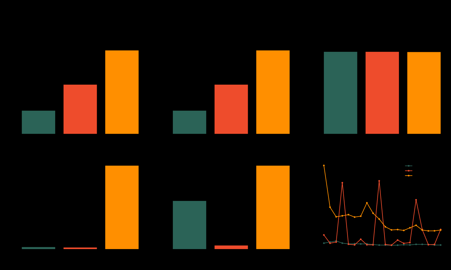
For the benchmark, all three frameworks ran CPU-only on the same sklearn Digits dataset, using the
same 80/20 train-test split, 64 → 128 → 64 → 10 MLP, GELU activations, AdamW, learning rate 0.001, batch size
32, and 20 epochs.
The results were interesting. picodl finished training in 1.59s, compared to 3.36s for PyTorch and 5.69s for TensorFlow/Keras. All three reached around 98% test accuracy, with picodl and PyTorch at 98.33% and TensorFlow at 98.06%.
Inference latency showed the expected tradeoff. For batch size 1, picodl averaged 0.130 ms, compared to 0.104 ms
for PyTorch. At batch size 128, picodl took 3.07 ms, while PyTorch took only 0.24 ms. This comparison,
visualised by matplotlib is attached below. Ultimately these results aren't meant to show that
picodl is faster than production frameworks. They're mainly a sanity check that a small numpy-based autograd
engine can train a real model and produce comparable results.
What you get instead is transparency. Every gradient comes from a derivative you can actually read, verify, and change. Debugging a shape mismatch means stepping through normal Python, and adding a new operation means writing its forward pass and derivative side by side.
picodl isn't trying to replace PyTorch. It's trying to make automatic differentiation less of a black box and more of something you can read from start to finish.
And who knows, it might become something more someday.
That's it for now, if you have any query, feel free to drop me an email at aanis@clipb.in.
Thanks for Reading,
Cheers!
> Go Back